Research · Multi-agent reinforcement learning
Learning Equilibria in Differential Games
A Julia package that lets a multi-agent reinforcement learning algorithm solve differential games, plus an exact stochastic linear-quadratic solver to check the learner against ground truth. Undergraduate research at CU Boulder under Dr. Vishala Arya and Bennet Outland.
Active · results below are current as of this writing
Two languages for the same problem
A differential game is several players, each with state evolving under a differential equation and each minimising its own cost, in continuous time. The solution concept is a Nash equilibrium: strategies from which no single player can improve by changing only its own. This framing is precise, and for the small and structured cases it is exactly solvable.
Multi-agent reinforcement learning describes the same situation, several agents optimising interdependent objectives, but finds strategies by learning rather than by solving. It scales to problems that have no closed form, at the cost of giving up any guarantee about what it converged to.
The project connects the two. Given a game specified in the formal language of differential games, apply a learning algorithm to it, and, where an exact answer exists, use that answer to measure how good the learned one is.
The package
The algorithm is MADDPG, an actor-critic method for continuous action spaces. Each agent’s actor sees only its own observations, so agents act independently once deployed. Each agent’s critic, used only during training, sees everyone’s observations and actions, which makes the environment look stationary from the critic’s point of view and removes the central pathology of multi-agent learning. The critics are discarded afterwards.
The implementation is in Julia. A game defined as a GameProblem is wrapped so it satisfies CommonRLInterface, which is the seam the whole design rests on: the bridge between game specification and learning environment is isolated in one file, and the neural network code never sees a task-specific detail. Four structures carry the package, an environment wrapper, a shared replay buffer, a per-agent actor and centralised critic, and a solver configuration holding the hyperparameters.
That bet has been tested twice. Going from a cooperative task to an adversarial one required no changes to the learning code at all, and neither did adding impassable polygon obstacles to the adversarial environment afterwards. The package is covered by a unit-test suite spanning the environment wrapper, the constraint modes, obstacle geometry and impassability, the reward structures, and a real gradient update.
Cooperative navigation
Three agents share a reward for covering three landmarks. An initial 1500-episode run beat the random-policy baseline by roughly 39 per cent and moved purposefully toward the landmarks, but held only two of the three, and the learning curve was still rising when training stopped. The obvious hypothesis was that the run was simply too short.
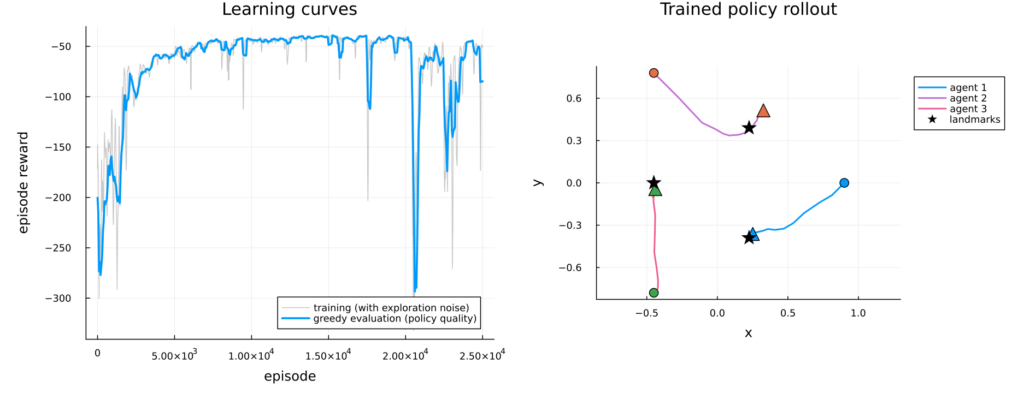
A 25,000-episode run answered that in both directions at once. The policy does get better: it now holds all three landmarks, and the trained rollout shows genuine task decomposition, with the agents splitting the landmarks between them and crossing the arena on a coordinated assignment rather than all converging on the nearest one. The curve then appeared flat from roughly episode 5000 onward.
That reading did not survive a closer look. Every episode in the run began from the same initial condition, because the environment reset to a fixed state, so what the evaluation measured was a single trajectory rather than a policy. Repeated with a fresh feasible start drawn for every episode, and each evaluation averaged over twenty held-out starts, the same task improves until roughly episode 13,000. The original run’s later behaviour was not a plateau either: after about episode 20,000 it destabilised, with roughly one episode in six falling below twice its own median, and that instability does not reproduce under randomised starts.
The useful result is therefore about measurement rather than about training length. A learning curve measured from one fixed initial condition describes a single path through the state space, and a Nash equilibrium of a differential game is defined over the whole of it.
Predator–prey pursuit and evasion
Cooperative navigation exercises only half of the algorithm’s design. With a shared reward the centralised critics never have to reconcile conflicting objectives. The pursuit–evasion extension supplies the other half: three predators chase a single prey that is thirty-three per cent faster, inside a hard-walled arena scattered with convex polygon obstacles. The wall and the obstacles are impassable by construction, enforced by projecting the state back out of them after every integration step, rather than merely penalised.
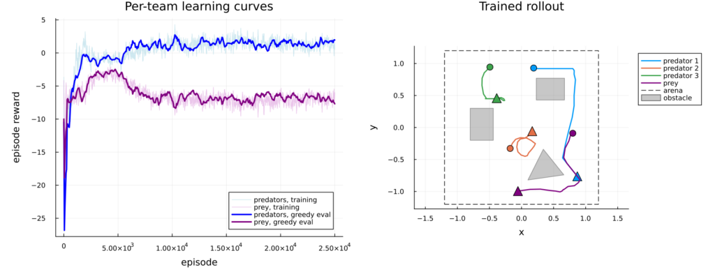
The most interesting result came from taking guidance away. The natural reward, and the one I used first, pays each predator for reducing its own distance to the prey. Under it the predators never caught the prey at all. Replacing it with the original paper’s sparse tag objective, where a predator is paid only for actual contact and that credit is shared across the whole team, took them to roughly twenty-seven per cent of every episode in contact.
The mechanism is worth spelling out, because it is the reverse of what reward shaping is supposed to do. A faster prey cannot be caught by a straight-line chase, and paying each predator for its own distance produces precisely a straight-line chase. The dense reward was not merely unnecessary, it was teaching the wrong strategy. Shared credit is the only structure under which hanging back to cut off an escape route pays, because it removes any advantage to being the predator who makes contact.
Both curves then flatten at around five to six thousand episodes out of twenty-five thousand, and by regression rather than by eye: the slope of the predator curve after episode six thousand carries a t-statistic of 0.11. Two candidate explanations were tested and rejected. Critic divergence was ruled out because the critic’s value estimates match those implied by the observed returns almost exactly. Exploration collapse was ruled out by lengthening the noise schedule so that exploration survives the whole run, and observing that the plateau did not move.
The flat curve turned out to be an artefact of how it was measured, in two compounding ways. Every episode started from one fixed initial condition, so the evaluation described a single trajectory rather than a policy. And episode reward in a two-sided game is a relative quantity: if the predators and the prey improve at the same rate the curve is exactly flat, so a flat curve cannot distinguish a learner that has stopped from two that are improving together.
Saving the policies every thousand episodes and playing the checkpoints against each other settles it. Rows are the predators at one point in training, columns the prey at another, so every entry holds one side fixed while the other varies. The predators’ scores against the full set of opponents rise from -8.2 to +4.0 across the run and the prey’s fall from +9.6 to -0.5, both with t-statistics beyond four in magnitude. Restricted to the window that looked plateaued, the predators gain 2.9 and the prey 2.2, which leaves 1.1 of net change in the self-play score. Learning never stopped. The two improvements were very nearly cancelling, and a self-play score was never capable of showing that.
A residual plateau does survive that correction: the predators’ cross-play scores climb steeply to about episode 4,000 and then flatten, and the same flattening appears when they are scored against an entirely different set of opponents, so it belongs to the predators rather than to the particular prey they trained against. Two mechanisms were proposed, and each made a falsifiable prediction. If the cause were replay-buffer staleness, shrinking the buffer fourfold should move the plateau to roughly episode 1,000. If it were the number of gradient updates, doubling the updates per environment step should move it to roughly 2,000. Neither moved. What the two experiments did establish is narrower and still useful: the smaller buffer produced worse policies on both sides, and doubling the gradient updates changed nothing at all for twice the compute.
Taking the shaping away
The arena and the obstacles are impassable by construction, and the predators cannot occupy the same point. Those facts were being enforced twice: once by the state projection, which makes them inviolable, and again by barrier costs inside the reward. Deleting the two redundant barrier terms, and changing nothing else, produced better policies on both sides.
That claim needs cross-play to make, and it is worth saying why I first got it wrong. Scored in self-play the unshaped run looks worse: 3.60 steps of contact per 25-step episode against the shaped run’s 4.34. I reported exactly that, and it was the same two-sided error this page has already described once. Played head to head the ordering reverses. The unshaped predators take 5.84 steps of contact off the shaped prey where the shaped predators take 4.34, and the unshaped prey holds the shaped predators to 2.16 where the shaped prey allows 4.34. Both rows and both columns agree. The self-play number was low precisely because both sides had improved and the improvements cancelled.
It also converged roughly six times faster, finishing its learning by about episode 4,000 where the shaped run climbs across all 25,000 and still does not reach the same strength. The mechanism is measured rather than inferred. Scoring the unshaped policy inside the shaped environment shows what it would have been charged for: its prey spends 11.86 of every 25 steps against the boundary, against 0.54 for the shaped prey. Backing into a corner is a good strategy when the wall is hard, because a cornered evader only has to defend a quarter circle. The arena barrier had been pricing the prey out of its best option, and the collision barrier had been charging the predators for closing in together. Neither term was guiding the learner toward the objective. Both were changing the game.
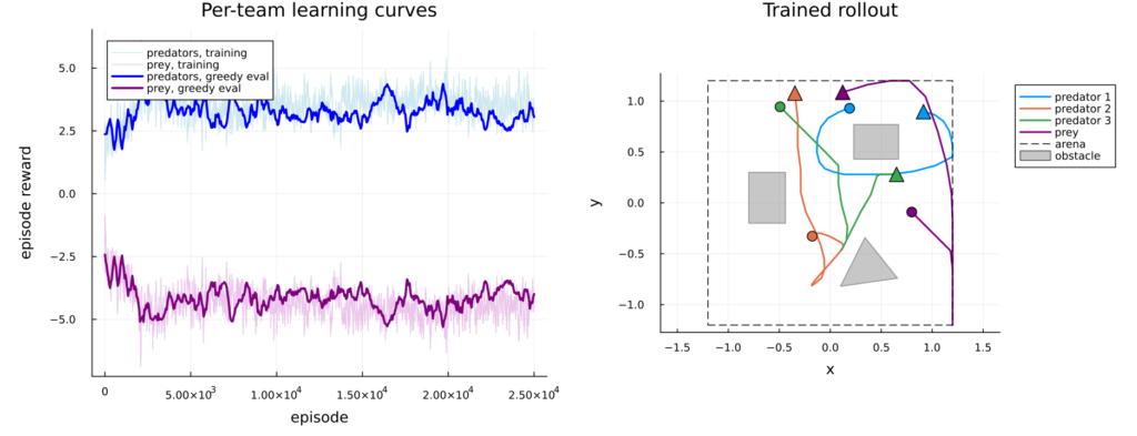
A second seed says the same thing. Repeating the unshaped run under a different random seed and playing it against the same shaped baseline gives 5.66 contact steps for its predators where the first seed gave 5.84, and its prey holds the shaped predators to 1.80 where the first gave 2.16. Both seeds finish learning by about episode 4,000. The size of the effect can be set against the size of the noise, because the two unshaped runs can be played against each other: they differ by 0.16 contact steps, against a shaped-to-unshaped gap of about 1.4, so the effect is roughly eight times the seed-to-seed variation. What is still untested is variation in the shaped baseline’s own seed, which is held fixed as the reference throughout.
Stochastic linear-quadratic games: ground truth
Everything above is measured against a random-policy baseline, which establishes that learning happened but not how close to optimal it got. Stochastic linear-quadratic games are among the few multi-agent problems whose feedback Nash equilibrium can be computed exactly, which makes them a yardstick for the learner. I implemented a solver for them, structured as a contribution to the base package, which declares a stochastic branch of its problem hierarchy but had no concrete implementation of it.
The solver is a coupled Riccati recursion covering additive, state-multiplicative and control-multiplicative noise. It produces a result that is worth stating on its own terms.
Under purely additive process noise, the stochastic feedback Nash gains are identical to the deterministic ones. Adding process noise does not change the controller at all. It makes the achieved cost worse by a computable amount, and nothing else.
This is certainty equivalence, and it matters practically because the expectation that adding noise will produce more robust gains is mathematically unfounded for that channel. Gains change only under multiplicative noise, whose terms survive differentiation with respect to the control, which is why the implementation covers those channels rather than additive noise alone.
Satellite formation flying
The solver was then put to work on a physical problem: three satellites assembling an along-track formation under Clohessy–Wiltshire–Hill relative orbital dynamics, perturbed by Gaussian process noise standing in for differential drag and unmodelled accelerations. Along-track slots are exact equilibria of those dynamics, so the assembled formation costs no fuel to hold and the problem stays purely linear-quadratic. That is what makes it a validation rather than a demonstration: nothing is approximated, so any disagreement between theory and simulation would be a bug rather than a modelling error.
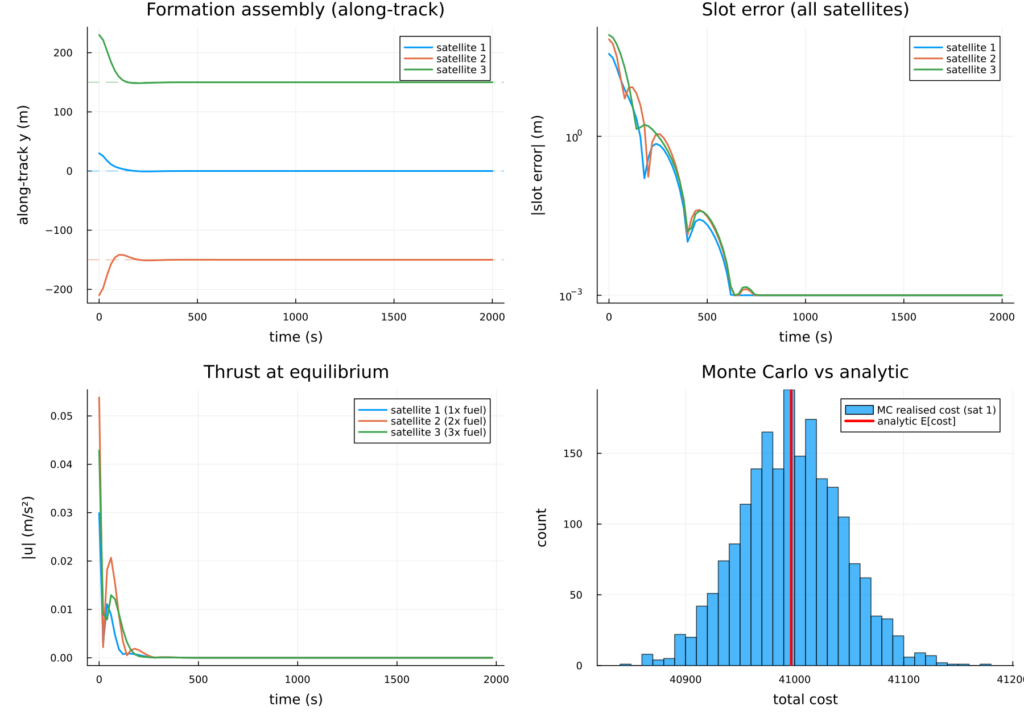
The analytic expected costs agree with a two-thousand-run Monte Carlo simulation to within half a standard error, the two figures coming from a backward Riccati recursion and a forward simulation with sampled noise that share no code between them. The equilibrium is also interpretable as a game rather than a control problem: each satellite pays for its own propellant, so the three optimising separately burn about six per cent more in total than a single controller commanding all of them would, and the satellite with the cheapest fuel performs most of the manoeuvre.
Verification
A Riccati recursion is easy to get subtly wrong and hard to check by inspection, so every test compares the solver against an independent computation rather than against itself: reduction to textbook LQR in the single-player case; the backward value function checked against an exact expected cost obtained by propagating the closed-loop mean and second moment forward, sharing no code, across all five noise regimes; certainty equivalence to machine precision; and the Nash property confirmed by a vanishing numerical gradient of each player’s cost with respect to its own gain.
All four checks were run first in an independent NumPy implementation, before any Julia was written, to separate errors of mathematics from errors of syntax. That paid off on the first execution of the Julia suite: every test capable of exposing an incorrect recursion passed immediately, and the only failures were in the test scaffolding itself, a reference LQR implementation missing a state-control cross term. Diagnosis was immediate rather than ambiguous, and the suite is stronger for it.
A certificate, not a convergence check
The solver is a finite backward pass rather than an iteration, so nothing converges in the fixed-point sense and there is no residual to watch. What can be certified is the Nash property itself. For each player, fix the others at the computed equilibrium, solve that player’s own optimal control problem exactly, and report the gap between the two costs. Zero for every player is the definition of a Nash equilibrium rather than evidence for one, and because the best response to affine opponents is itself affine under linear dynamics and quadratic costs, a zero gap certifies against all deviations rather than only affine ones.
Run on the three-satellite formation problem across all three noise channels, every player’s gap comes out within 7.3 x 10⁻¹² of zero, and each player’s equilibrium cost agrees to the last digit with a second computation sharing no code with the first. Two cross-checks frame the result. Additive noise leaves the gains identical to the deterministic ones to exactly zero, which is certainty equivalence appearing as a number rather than as an argument. A ten per cent thruster gain error moves them by 1.035 x 10⁻³, which is why the multiplicative channels are the ones worth benchmarking a learner against. And a deliberate perturbation of one player’s gains registers as a strictly positive gap, which is the check that the measurement is capable of failing at all.
Where it goes next
The exact exploitability machinery is now built and run, which turns the next step from a design question into a measurement: the same linear-quadratic game solved both ways, learner and exact solver, with the gap between them as the result. That would be the first measurement of optimality rather than of improvement anywhere in the project. Building it where it is exact is also what makes an approximate version trustworthy on the problems where no exact answer exists, which is every problem in the first half of this page.
The guided-policy-search wrapper has started. Guided policy search solves a local linear-quadratic problem at every iteration, so that is the seam: make the local solver a constructor argument and the same outer loop becomes classic guided policy search, guided policy search for deterministic differential games, or guided policy search under multiplicative uncertainty, with nothing else rewritten. The local step is implemented and tested. Single-player LQR, deterministic Nash and stochastic Nash are interchangeable arguments, and selecting the stochastic path with purely additive noise reproduces the deterministic path to exactly zero, so certainty equivalence doubles as a test of the plumbing. The outer loop is not written, and the piece of it with real content is the trust region: single-agent guided policy search adapts its step size by comparing predicted against actual cost improvement, and a game has no scalar that ought to decrease monotonically.
Beyond that, a risk-sensitive variant of the recursion, which would reuse the same backward pass, and resolving where the solver belongs in the ecosystem, given that the base package currently holds no concrete solvers of its own.